Let’s take a random walk down a Random Forest path!

Scientists have always been looking to explain the world through observations and data. But what has always fascinated me about life, is that randomness, one way or another, will always play its part.

At least that’s what I’d like to think Tim Kam Ho, a computer scientist at IBM Watson, had in mind when she first created Random Forest.

This post will cover the basics of the Random Forest model and the concepts that underlie it.

Decision Trees

A decision tree is a flow-chart-like tree structure, where each internal node represents a test/question on an attribute, each branch represents an outcome of the test/question, and leaf nodes represent different class breakdowns.

Here’s an example of a decision tree surrounding a question that I hope I’ll be soon considering: “Should I accept a new job offer?”

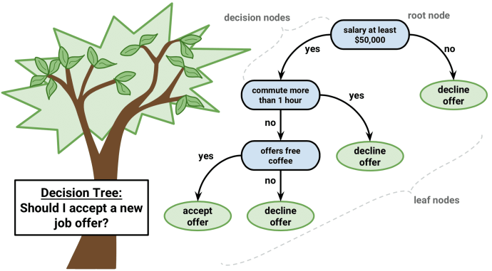
In this example, the first decision node that I consider is “Does the salary pay at least $50,000?” If the answer is no, than the tree follows the “No” branch, leading me to decline the offer. However, if the answer is yes, then the tree follows the “Yes” branch and I consider an additional decision node of “Is the commute longer than one hour?” Playing out this next decision node is a similar yes or no question, if the answer is “Yes” to this question, than I would decline the job offer, if the answer is “No,” I continue on down the decision tree path.

The ultimate objective here is to arrive at a decision to a yes or no question. However, decision trees have many plausible applications and can be applied to more than just binary decisions. They can be used for a wide array of classification and regression tasks (though it’s far more commonly used in classification tasks).

For tasks that aren’t as straight-forward as yes or no questions, we’ll see that the purpose of each decision node is to achieve the greatest amount of information gained. Ideally, at each decision, the aim is to create nodes with the greatest amount of purity (or data that belongs to the same class).

On a side note, decision trees suffer from issues of high variance, which we’ll see how Random Forest combats that factor later on.

Explaining Information Gain - Gini and Entropy

One of the most important factors in using any type of decision tree is establishing optimal splits at each branch. To do this, we objectively measure information gain via gini or entropy. The formulas for each are as such:

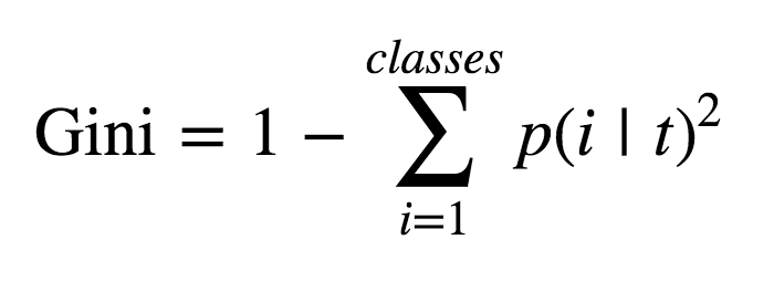
The key takeaway here is that both are more or less the same measurement of informational gain that a computer will consider when deciding how to create a decision node. Computationally it will break apart its data into consecutively smaller, and hopefully more pure, nodes until it arrives at an completely ‘pure’ node. In other words, a node where each data point is of the same classification.

The computer will then take gini or entropy and apply it to this information gain formula (where H = gini or entropy, Nj = # of classes, N = total number of observations, and child = proportion of class observations):

A simplified version of this formula is:

Bootstrapping

Another key idea applied in Random Forest models is bootstrapping. Bootstrapping is the practice of randomly sampling a distribution with replacement. Replacement means that we can pick out an individual sample (marble), then place that marble back into the population. In other words, it’s possible that we could select the same marble more than once. Based off of our sample observations, we can then calculate the mean based off of all those samples.

For example, let’s say we have a population of 9 colored marbles: 3 blue, 2 orange, 2 yellow, and 2 green. And we’d like to know how many marbles there are of each color, but we can’t directly count them. We could use bootstrapping to repeatedly sample the collection of marbles, and then based off of those samplings, try to figure out the actual distribution of colors.

A visualization of this:

This image effectively visualizes sampling with replacement as well. Notice in bootstrap example 1, there are 3 yellow marbles, but there’s actually only 2 yellow marbles total in our population, so one of the yellow marbles was sampled more than once.

Using this example, the calculated means of each color are: Blue = 3.67, Yellow = 2.67, Green = 1.33, & Orange = 1.33. The more bootstrap samples we collect, the closer our calculated means will be to their actual values.

In my next section, I’ll explain how bootstrapping can be applied to machine learning on a more significant scale.

Ensemble Method & Bagging

An ensemble method is a technique that combines the predictions from multiple machine learning algorithms together to make more accurate predictions than any individual model. The idea being that multiple ‘weak learner’ models can be combined and averaged out to create one ‘strong learner’ model. This is loosely referred to as “the wisdom of the crowd.”. To apply an ensemble method, we must apply the concept of bagging.

Bootstrap aggregating, or bagging, is the application of bootstrapping to multiple, high-variance machine learning algorithms.

A visualization of these ideas:

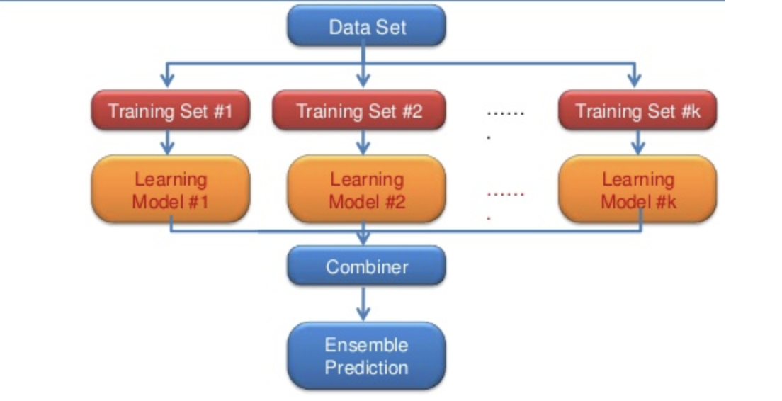
In this example, we take a set of data and create training sets off of it. We then create models off of these individual training sets, and then aggregate those models collective predictions (for regression tasks) or vote on the class (for classification tasks) to create an ensemble prediction.

As I’ll explain in my next section, the Random Forest ensemble method takes this idea a step further.

Random Forest

Random Forest is a commonly-used ensemble learning method for both classification and regression tasks. It operates by creating multiple decision trees, sampling n cases, using M total features. However, randomness is introduced by only allowing m random variables to be selected at each node, where m < M. m is held constant while the forest is built out.

If we did not force the computer to sample random variables, it would generally choose the same variables to split on repeatedly. Thus creating decision trees that are highly correlated with each other and don’t have much predictive power, collectively, over any individual decision tree.

In other words, this is to decorrelate our trees from each other, decrease variance, and reduce issues of overfit to increase the overall quality of our ensemble model’s prediction.

A visualization of this, after our trees are built out, using an individual instance of our data:

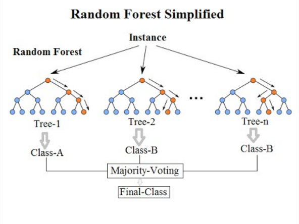
An instance is passed through each random forest iteration, each tree decides what it would classify that instance as, and then they collectively vote on what the final class is.

And that’s pretty much it! Hopefully you found this post edifying on the subject of Random Forests! Thanks for reading!

Here’s another random picture of a Random Forest!